
Regularization Methods Complete Guide: From Ridge to Elastic Net

Regularization methods are the cornerstone of robust machine learning, helping practitioners combat overfitting, improve model generalizability, and handle real-world data challenges like multicollinearity and high dimensionality. In this comprehensive guide, we will demystify regularization techniques from the ground up — exploring Ridge, Lasso, and Elastic Net, digging into their mathematical foundations, geometric intuitions, and practical applications. Whether you’re a data scientist, machine learning engineer, or an enthusiast, this article will provide actionable insights, code examples, and case studies to make regularization work for you.
1. Overfitting Problem: Mathematical Explanation
At the heart of many machine learning challenges is the problem of overfitting. Overfitting occurs when a model learns not only the underlying patterns in the training data but also the noise, resulting in poor generalization to unseen data.
Mathematically, consider a dataset with $n$ observations: $(\mathbf{x}_i, y_i)$ for $i=1,\ldots,n$, where $\mathbf{x}_i \in \mathbb{R}^p$ (feature vector) and $y_i$ is the target. Suppose we fit a linear model:
$$ \hat{y}_i = \mathbf{x}_i^\top \boldsymbol{\beta} $$
The Ordinary Least Squares (OLS) estimator finds $\boldsymbol{\beta}$ by minimizing the residual sum of squares (RSS):
$$ \min_{\boldsymbol{\beta}} \sum_{i=1}^n (y_i - \mathbf{x}_i^\top \boldsymbol{\beta})^2 $$
If $p$ (number of features) is large or the model is too flexible, it can fit the training data perfectly ($RSS \to 0$), but this leads to high variance and poor predictive performance on new data.
2. Bias-Variance Tradeoff Visualization
The bias-variance tradeoff explains why overly complex models can overfit, while overly simple models can underfit:
- Bias: Error due to overly simplistic assumptions.
- Variance: Error due to sensitivity to small fluctuations in the training set.
The expected prediction error can be decomposed as:
$$ \mathbb{E}\left[(y - \hat{f}(\mathbf{x}))^2\right] = \text{Bias}^2 + \text{Variance} + \text{Irreducible Error} $$
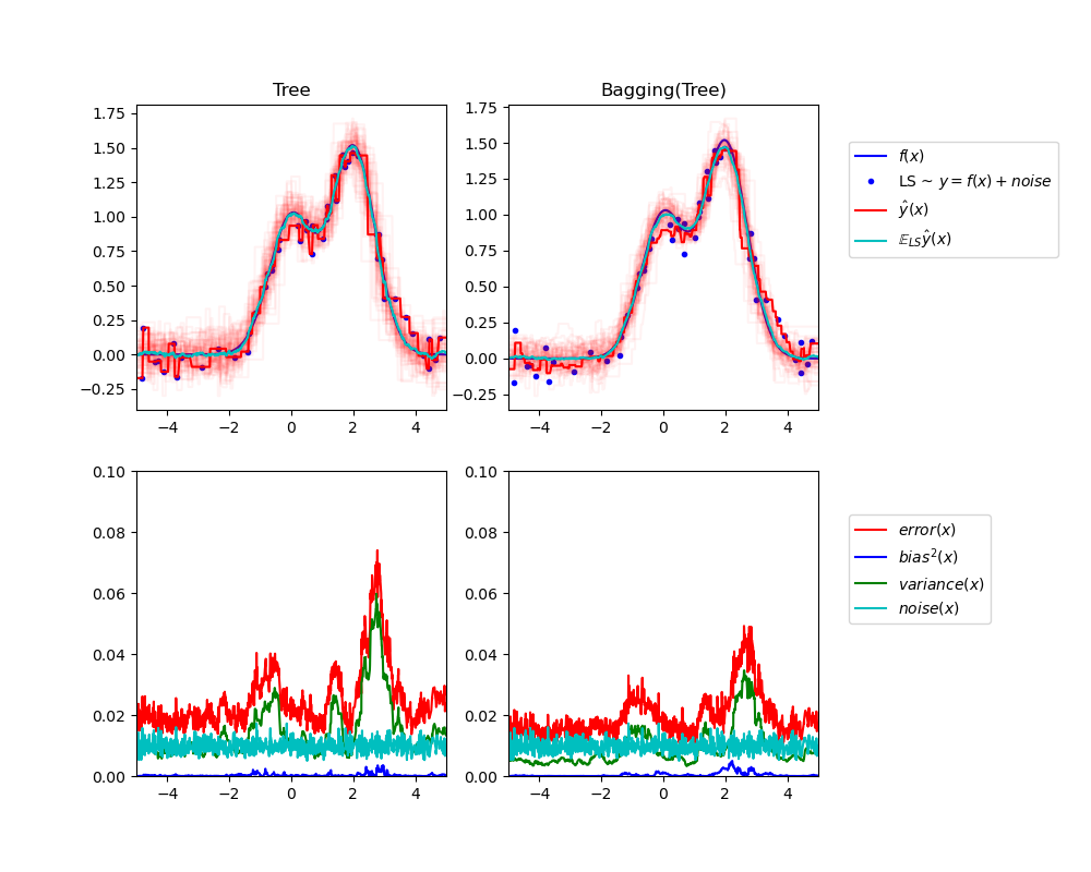
Regularization helps to control model complexity, striking a balance between bias and variance.
3. Ridge Regression: Derivation and Properties
Ridge regression (also known as Tikhonov regularization) addresses overfitting by penalizing large coefficients. The objective function is:
$$ \min_{\boldsymbol{\beta}} \sum_{i=1}^n (y_i - \mathbf{x}_i^\top \boldsymbol{\beta})^2 + \lambda \|\boldsymbol{\beta}\|_2^2 $$
Where $\|\boldsymbol{\beta}\|_2^2 = \sum_{j=1}^p \beta_j^2$ and $\lambda \geq 0$ is the regularization parameter.
The closed-form solution for Ridge regression is:
$$ \boldsymbol{\hat{\beta}}_{ridge} = (\mathbf{X}^\top \mathbf{X} + \lambda \mathbf{I})^{-1} \mathbf{X}^\top \mathbf{y} $$
- Properties:
- It shrinks coefficients towards zero but never exactly zero.
- Handles multicollinearity well.
- Bias increases, variance decreases as $\lambda$ increases.
4. Lasso Regression: Geometric Interpretation
Lasso regression (Least Absolute Shrinkage and Selection Operator) uses an L1 penalty:
$$ \min_{\boldsymbol{\beta}} \sum_{i=1}^n (y_i - \mathbf{x}_i^\top \boldsymbol{\beta})^2 + \lambda \|\boldsymbol{\beta}\|_1 $$
Where $\|\boldsymbol{\beta}\|_1 = \sum_{j=1}^p |\beta_j|$.
Geometric Intuition:
- The constraint region for Lasso is a diamond (in 2D), while for Ridge, it's a circle.
- The corners of the diamond (L1 ball) increase the likelihood that solutions will hit axes, resulting in some coefficients being exactly zero (feature selection).
5. Elastic Net: Combining Ridge and Lasso
Elastic Net blends Ridge and Lasso penalties:
$$ \min_{\boldsymbol{\beta}} \sum_{i=1}^n (y_i - \mathbf{x}_i^\top \boldsymbol{\beta})^2 + \lambda_1 \|\boldsymbol{\beta}\|_1 + \lambda_2 \|\boldsymbol{\beta}\|_2^2 $$
Or, using a mixing parameter $\alpha$:
$$ \min_{\boldsymbol{\beta}} \sum_{i=1}^n (y_i - \mathbf{x}_i^\top \boldsymbol{\beta})^2 + \lambda \left[ \alpha \|\boldsymbol{\beta}\|_1 + (1-\alpha) \|\boldsymbol{\beta}\|_2^2 \right] $$
- When $\alpha=1$, Elastic Net is equivalent to Lasso.
- When $\alpha=0$, it is Ridge.
- Suitable when there are highly correlated features (groups of predictors).
6. Bayesian Interpretation of Regularization
Regularization can be understood from a Bayesian perspective:
- Ridge regression corresponds to a Gaussian prior on $\boldsymbol{\beta}$: $$ p(\boldsymbol{\beta}) \propto \exp\left(-\frac{\lambda}{2}\|\boldsymbol{\beta}\|_2^2\right) $$
- Lasso regression corresponds to a Laplace prior on $\boldsymbol{\beta}$: $$ p(\boldsymbol{\beta}) \propto \exp\left(-\lambda \|\boldsymbol{\beta}\|_1\right) $$
This interpretation allows for probabilistic modeling and helps connect regularization to broader statistical frameworks.
7. Computational Algorithms: Coordinate Descent
For Lasso and Elastic Net, the penalty is non-differentiable at zero, making closed-form solutions infeasible. Coordinate Descent is a widely used algorithm for these problems.
- Iteratively optimizes each parameter $\beta_j$ while holding others fixed.
- Efficient for high-dimensional, sparse problems.
# Pseudocode
for iteration in range(max_iter):
    for j in range(p):
        # Update beta_j based on partial residuals
        beta_j = update_rule()
8. Python Implementation: sklearn Examples
Scikit-learn offers easy-to-use implementations for all regularization methods. Below are brief examples for Ridge, Lasso, and ElasticNet:
from sklearn.linear_model import Ridge, Lasso, ElasticNet
from sklearn.datasets import make_regression
from sklearn.model_selection import train_test_split

# Generate synthetic data
X, y = make_regression(n_samples=100, n_features=20, noise=0.1, random_state=42)
X_train, X_test, y_train, y_test = train_test_split(X, y, random_state=42)

# Ridge Regression
ridge = Ridge(alpha=1.0)
ridge.fit(X_train, y_train)
print("Ridge R^2:", ridge.score(X_test, y_test))

# Lasso Regression
lasso = Lasso(alpha=0.1)
lasso.fit(X_train, y_train)
print("Lasso R^2:", lasso.score(X_test, y_test))

# Elastic Net
elastic = ElasticNet(alpha=0.1, l1_ratio=0.7)
elastic.fit(X_train, y_train)
print("Elastic Net R^2:", elastic.score(X_test, y_test))
9. Cross-Validation for Lambda Selection
Choosing the optimal regularization parameter ($\lambda$ or alpha) is critical. Cross-validation is the standard method:
- Split data into training and validation sets.
- Train models for a range of $\lambda$ values.
- Select the $\lambda$ with the best validation performance.
from sklearn.linear_model import LassoCV

# Lasso with cross-validation
lasso_cv = LassoCV(alphas=[0.01, 0.1, 1, 10], cv=5)
lasso_cv.fit(X_train, y_train)
print("Best alpha:", lasso_cv.alpha_)
print("Test R^2 with best alpha:", lasso_cv.score(X_test, y_test))
10. Feature Selection with Lasso
A key advantage of Lasso is automatic feature selection:
- Lasso tends to set some coefficients exactly to zero, effectively removing less relevant features.
- This is particularly useful in high-dimensional datasets (e.g., genomics, text).
import numpy as np

lasso = Lasso(alpha=0.1)
lasso.fit(X_train, y_train)
selected_features = np.where(lasso.coef_ != 0)[0]
print("Selected feature indices:", selected_features)
11. Multicollinearity Solutions with Ridge
Multicollinearity (high correlation between features) inflates variance of OLS estimators. Ridge regression mitigates this by adding a penalty term, making $\mathbf{X}^\top \mathbf{X} + \lambda \mathbf{I}$ invertible even if $\mathbf{X}$ is not of full rank.
- Ridge distributes the effect across correlated features rather than arbitrarily assigning large positive/negative weights as OLS might.
12. Case Study: High-Dimensional Financial Data
Consider a stock return prediction task with 1,000 features (technical indicators) and 500 samples. OLS will overfit; Lasso and Elastic Net provide sparse, interpretable models.
from sklearn.linear_model import ElasticNetCV

# Simulate high-dimensional data
X_fin, y_fin = make_regression(n_samples=500, n_features=1000, noise=0.5, random_state=42)
elastic_cv = ElasticNetCV(l1_ratio=[.1, .5, .7, .9, .95, 1], cv=5)
elastic_cv.fit(X_fin, y_fin)
print("Optimal l1_ratio:", elastic_cv.l1_ratio_)
print("Optimal alpha:", elastic_cv.alpha_)
print("Test R^2:", elastic_cv.score(X_fin, y_fin))
Elastic Net outperforms Ridge and Lasso when there are groups of correlated predictors.
13. Case Study: Text Classification with Regularization
In text classification (e.g., spam detection), features are word counts or TF-IDF values, resulting in thousands of sparse features.
from sklearn.feature_extraction.text import TfidfVectorizer
from sklearn.linear_model import LogisticRegressionCV

corpus = [
    "Buy cheap watches now",
    "Meeting scheduled at 10am",
    "Congratulations, you won a prize!",
    "Lunch with project team"
]
labels = [1, 0, 1, 0]  # 1: Spam, 0: Not Spam

vectorizer = TfidfVectorizer()
X_text = vectorizer.fit_transform(corpus)

logreg_cv = LogisticRegressionCV(
    Cs=10, penalty='l1', solver='saga', cv=3, scoring='accuracy', max_iter=1000
)
logreg_cv.fit(X_text, labels)
print("Best C (inverse regularization):", logreg_cv.C_[0])
print("Coefficients shape:", logreg_cv.coef_.shape)
L1 regularization (Lasso) for logistic regression selects a small, interpretable set of predictive words.
14. Extensions: Group Lasso, Adaptive Lasso
- Group Lasso: Penalizes groups of coefficients, encouraging sparsity at the group level. Useful when features are naturally grouped (e.g., polynomial terms, categorical variables).
$$ \min_{\boldsymbol{\beta}} \sum_{i=1}^n (y_i - \mathbf{x}_i^\top \boldsymbol{\beta})^2 + \lambda \sum_{g=1}^G \|\boldsymbol{\beta}_g\|_2 $$
- Adaptive Lasso: Improves variable selection consistency by assigning different weights to different coefficients.
$$ \min_{\boldsymbol{\beta}} \sum_{i=1}^n (y_i - \mathbf{x}_i^\top \boldsymbol{\beta})^2 + \lambda \sum_{j=1}^p w_j |\beta_j| $$
15. Regularization in Neural Networks
Regularization is crucial in neural networks to prevent overfitting due to their high capacity:
- L2 Regularization (Weight Decay): Adds $\lambda \|\mathbf{W}\|_2^2$ to the loss function.
- L1 Regularization: Adds $\lambda \|\mathbf{W}\|__2$ to the loss function, encouraging sparsity in neural network weights.
- Dropout: Randomly sets a fraction of activations to zero during training, which acts as a form of regularization by preventing co-adaptation of feature detectors.
Mathematically, for a neural network with weights $\mathbf{W}$ and loss function $\mathcal{L}(\mathbf{W})$, L2 regularization modifies the loss as:
$$ \mathcal{L}_{\text{reg}}(\mathbf{W}) = \mathcal{L}(\mathbf{W}) + \lambda \|\mathbf{W}\|_2^2 $$
L1 regularization modifies it as:
$$ \mathcal{L}_{\text{reg}}(\mathbf{W}) = \mathcal{L}(\mathbf{W}) + \lambda \|\mathbf{W}\|_1 $$
Regularization helps neural networks generalize better, especially on limited data or when the network is deep/wide.
16. Common Misconceptions Clarified
- “Regularization always improves accuracy.”
Not necessarily. In some cases, too much regularization can underfit the data, increasing bias and reducing accuracy. - “Ridge regression eliminates irrelevant features.”
No, Ridge regression shrinks coefficients but rarely sets them exactly to zero. For feature elimination, Lasso or Elastic Net are preferred. - “Lasso is always better than Ridge.”
Not always. Lasso works well when only a few features are relevant. Ridge is superior when all features are useful but need regularization due to multicollinearity. - “Elastic Net is just a combination; it’s never best.”
In fact, Elastic Net often outperforms both Ridge and Lasso when features are highly correlated or when there are more predictors than samples. - “Regularization parameter ($\lambda$) selection is not important.”
Incorrect. Choosing $\lambda$ by cross-validation or Bayesian methods is critical to achieving optimal performance.
17. Interview Questions with Solutions
| Question | Solution/Explanation |
|---|---|
| 1. Why can't Lasso regression be solved with a closed-form solution like Ridge? | Because the L1 penalty introduces non-differentiability at zero, making the optimization problem non-smooth. As a result, iterative algorithms like coordinate descent are needed. |
| 2. Given a dataset with $p \gg n$, which regularization method(s) would you use and why? | Lasso or Elastic Net, since they perform feature selection and can handle high-dimensional data where the number of predictors exceeds the number of samples. |
| 3. What is the effect of increasing $\lambda$ in Ridge regression? | As $\lambda$ increases, coefficients shrink more towards zero, increasing bias but reducing variance, which can help prevent overfitting. |
| 4. How does Elastic Net help with correlated features? | Elastic Net can select groups of correlated features together, unlike Lasso, which tends to select only one from a group of highly correlated predictors. |
| 5. What is the Bayesian interpretation of Ridge regression? | Ridge regression corresponds to assuming a Gaussian prior with zero mean for the coefficients, i.e., $p(\boldsymbol{\beta}) \sim \mathcal{N}(0, \sigma^2/\lambda \mathbf{I})$. |
| 6. How does cross-validation help in regularization? | By evaluating model performance on validation folds for different $\lambda$ values, cross-validation helps select the regularization parameter that yields the best generalization. |
| 7. Can Lasso regression select more features than the number of samples? | No. In the case where $p > n$, Lasso can select at most $n$ features before coefficients start to become zero due to the geometry of the solution. |
Conclusion
Regularization methods are vital tools for building robust, interpretable, and high-performing machine learning models. Ridge, Lasso, and Elastic Net each address different challenges—be it multicollinearity, feature selection, or correlated predictors. By understanding their mathematical foundations, computational algorithms, and practical applications, you can make informed choices tailored to your data science problems. Cross-validation and diagnostic tools further enhance the ability to tune these methods for optimal performance.
Whether you’re working with financial data, text, or neural networks, mastering regularization will elevate your modeling skills and results.
Further Reading
- Scikit-learn: Ridge Regression
- Scikit-learn: Lasso
- Scikit-learn: Elastic Net
- Bias-Variance Tradeoff (CMU Lecture Notes)
- L1 vs L2 Regularization
