When running advertising campaigns, businesses want to understand how ads impact sales over time. Two key phenomena affect this relationship:

1. Ad effects don’t disappear instantly → There is a Carryover Effect. Ads don’t just impact the week they are shown. Their effect lingers over time. A simple regression media mix model fails to capture this effect. (In this article we have modeled this using Adstock function)
2. More spending doesn’t always mean more sales → There is Diminishing Returns. Doubling the ad spend will most likely not double the sales. More spend helps initially but loses efficiency over time. A simple regression media mix model fails to capture this effect. (In this article this effect is modeled using Hill Function)

Data Overview

We assume that we have weekly data (by market) for weeks from t = 1, . . . , T. There are M media channels in the media mix, and x{t,m} is the media spend of channel m at week t. The actual sales (or log transformed sales) at time t is given by y(t), whereas our estimate is given by y’(t). We put all other non-media variables into another group z (control variables). This includes all other relevant factors such as price, product distribution, seasonality, etc. which are likely to affect the sales. We use z{t,c} to denote the value of the c-th control variable at week t.

Model Specification

The core idea is to model sales response y’(t) as a function of:

• Media spend across different channels (TV, digital, search, etc.).
• Control variables (price, seasonality, product distribution).
• Random noise to account for unexplained variation.

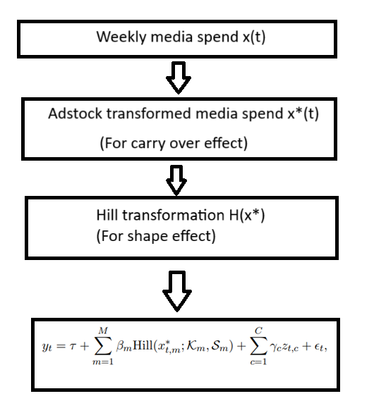
Here’s an outline of the modelling approach. We take the weekly media spend data, transform it using the Adstock function (to the model the carryover effect) first and then transform the result through the Hill function (to model the shape effect). Finally, we use the output of the Hill function as input into our regression model. The details of each function and the purpose they serve are described in the sections below.

The general form of the model is:

where:

• y(t)​ = Sales (or log-transformed sales) at time t.
• x{t,m} = Media spend for channel m at time t.
• f(x{t,m}) = Media spend transformation, accounting for carryover and shape effects. This is done through two transformations — Adstock function and Hill function.
• z{t,c} = Control variables (price, seasonality, etc.).
• βm​, γc​ = Coefficients for media and control variables.
• τ = Baseline sales.
• ϵ(t)​ = Random noise.

This is not a linear regression model (because of the Adstock and Hill function) so we’ll not be able to use LSE to find the parameters.

Carryover Effect (Adstock Transformation)

Advertising does not just impact sales in the current week; its effects carry over into future weeks. This is captured by the adstock function.

Adstock Transformation Formula

where:

• L = Maximum number of weeks the ad effect lasts.
• wm(l) = Weight function that determines how media spend at week t−l contributes to sales at week t.

Two Types of Adstock Functions

1. Geometric Adstock (Standard Decay)

• Retention rate αm​ controls how fast ad effects decay.
• Example: If αm=0.8, an ad shown this week still has 80% of its effect next week.

1. Delayed Adstock (Peak Effect Occurs Later)

• θm​ determines when the ad effect peaks.
• More realistic for brand awareness campaigns, where an ad’s impact might take time to build.

Comparison:

• Geometric adstock assumes the effect starts strong and fades gradually.
• Delayed adstock allows for a lagged peak, which is useful for ads that take time to influence consumers.

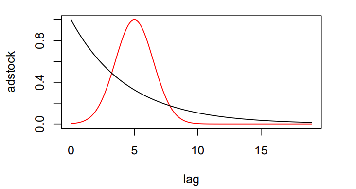
Geometric (black) and Delayed (red) Adstock function example.

Shape Effect (Diminishing Returns)

Ad spend does not have a linear effect on sales. If you keep increasing spend, eventually you hit diminishing returns.

Hill Function (Saturation Effect)

where:

• Km​ = Half-saturation point (spend level at which sales reach 50% of max effect).
• Sm​ = Shape parameter (controls how steeply the curve flattens).

The final transformation of media spend is: βm⋅Hill(xt,m)

How It Works:

• At low spend: The function is nearly linear.
• At high spend: Sales flatten out (diminishing returns).
• If Sm>1: More “S”-shaped (convex at low spend, concave at high spend).
• If Sm<1: More concave (flattens quickly).

Alternative Shape Transformations

• Reach Transformation (simpler alternative to Hill function):

• Used in TV campaign reach estimation.
• Works well when Sm is hard to estimate.

Parameters to Estimate

The key parameters in the model are:

A. Adstock Parameters (Carryover Effect)

• αm​ (Retention Rate): Controls how fast advertising effects decay over time.
• θm (Delay Parameter): Controls how long it takes for an ad to reach its peak effect.

B. Shape Parameters (Diminishing Returns)

• Km​ (Half-Saturation Point): Spend level at which 50% of the maximum response is reached.
• Sm: Controls how quickly ad effectiveness saturates.

C. Regression Parameters

• βm​ (Media Effect Coefficients): How much each media channel contributes to sales.
• γc​ (Control Variable Coefficients): The effects of price, seasonality, etc.
• τ (Baseline Sales): The expected sales without media spend.

Bayesian Estimation Approach

Instead of solving for parameters directly, we use Bayesian inference to estimate them from the posterior distribution.

Define the Likelihood Function

The likelihood function represents how well the model explains the data. The likelihood function for the above model is given by:

where Φ is the set of all parameters to estimate.

Define Prior Distributions

Since we are using Bayesian estimation, we specify prior beliefs about the parameters:

Compute the Posterior Distribution

Using Bayes’ Theorem:

• Likelihood p(y∣X,Z,Φ): How well the model explains the data.
• Prior p(Φ): Our initial beliefs about the parameters.

Since this does not have a closed-form solution, we use sampling methods to approximate the posterior.

Sampling with Markov Chain Monte Carlo (MCMC)

Why MCMC?

• The model has nonlinear transformations, making direct estimation impossible.
• MCMC allows us to sample from the posterior distribution.

Common MCMC Methods

1. Gibbs Sampling

• Iteratively samples each parameter while keeping others fixed.
• Works well when conditional distributions are known.

1. Hamiltonian Monte Carlo (HMC)

• Uses gradients to explore the parameter space more efficiently.
• More efficient than Gibbs sampling for complex models.

ROAS (Return on Ad Spend)

Once we have the model parameters, ROAS can be estimated using the below formula:

• Compute predicted sales y(t)​ under normal media spend.
• Set spend of media channel m to zero and recompute y(t)(x{t,m=0})​.
• ROAS is the change in sales per dollar spent.

Optimizing Media Mix

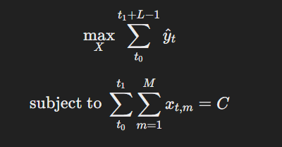
We can estimate the media spend allocation X∗ that maximizes sales under a budget constraint by solving the following constrained optimization:

Key Results

Simulation Studies:

• Bayesian models work well with large data but produce biased results when data is small.
• The choice of priors has a big impact.
• ROAS (Return on Ad Spend) estimates are more reliable for high-budget channels.

Practical Applications

• Calculate Return on Ad Spend (ROAS): Measures how much revenue is generated per dollar spent on ads.
• Find the Optimal Media Mix: Identifies how to allocate budgets across different channels to maximize sales.
• Understand Ad Effectiveness Over Time: Helps marketers adjust campaigns based on how long ads continue to influence sales.

References

Bayesian Methods for Media Mix Modeling with Carryover and Shape Effects by Yuxue Jin, Yueqing Wang, Yunting Sun, David Chan, Jim Koehler Google Inc. 14th April 2017

This article was originally posted on Medium: https://medium.com/@adnan.tamimi2290/bayesian-approach-to-media-mix-modelling-804374684840